Implementing HNSW index (Part 1)

Every time you send a prompt to an LLM-powered app, there’s a good chance something happens before the model even sees your message: the system takes your prompt, converts it into a vector, searches a database for the most similar vectors, fetches the matching documents, and then hands everything to the model as context. That’s RAG in a nutshell, and it happens on basically every query in production AI systems today. The search part is what this post is about.

Vectors here are just lists of numbers. Tools called embedding models take raw input (a sentence, an image, a PDF chunk, whatever) and compress it into a fixed-size list of floats where similar inputs end up with numerically similar lists. The search problem then becomes: given this query vector, find the closest ones in a dataset that might have tens or hundreds of millions of entries.

The naive approach is to compare the query against every single entry in the database (linear scan). Once your dataset grows to millions of entries, linear scan becomes the bottleneck, and at serious scale it just falls apart. This is why vector indexes exist, specifically approximate nearest neighbor (ANN) indexes. The idea is simple: you don’t always need the exact nearest neighbor; close enough is fine, and that relaxation is what makes fast search possible. You’ll find these inside Pinecone, Weaviate, Qdrant, and pgvector. The most widely used one today is HNSW (Hierarchical Navigable Small World), and that’s what this series covers. Part 1 builds the mental model. Part 2 gets into the algorithms and implementation details from VortexDB, a vector database in Rust we’re building at SDSLabs.

Where HNSW comes from

HNSW is basically two older data structures combined. Both had interesting ideas but each had a problem that made them not good enough on their own.

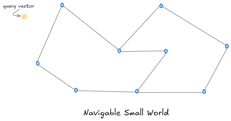
NSW — Navigable Small World

NSW is a graph where each vector is a node, and each node is connected to a few of its nearest neighbors. To find vectors similar to a query, you pick a starting node and keep jumping to whichever connected neighbor is closest to your query. Repeat until no neighbor brings you closer. It’s like asking “who do you know that might know this person?” and following that chain of referrals. Because of the small world property, you don’t need many hops to get anywhere in the graph, even if it has millions of nodes — similar to how you’re connected to almost any person in the world through just a handful of mutual friends.

NSW has two real problems though. The first is local minima. The greedy walk stops the moment no neighbor is closer to the query than the current node. But “closer” only considers the nodes you’re directly connected to. The actual nearest neighbor might exist somewhere in the graph but simply isn’t reachable from where you got stuck. You’d need a different starting point or a longer-range connection to get there, and NSW has neither.

The second problem is hub nodes. When the graph is first being built and only has a few nodes, every new insertion naturally connects to those few existing nodes since there’s no one else nearby. By the time the graph has millions of nodes, those early nodes have accumulated connections from thousands of later insertions. Every search ends up passing through these hubs regardless of the actual query, just because they’re connected to everything. This makes the graph increasingly unbalanced as it grows.

Skip Lists

A skip list is a sorted linked list with multiple layers stacked on top of each other. The bottom layer has every element in sorted order. Each layer above keeps only a random subset of elements from the layer below, so it has fewer nodes but bigger gaps between them.

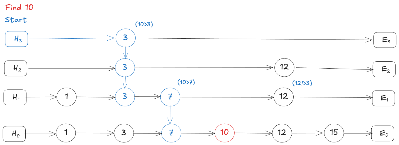
To search, you start at the top-left node and scan right. When the next node would overshoot your target, you drop down a layer and continue. This way you skip over large chunks of the list early on and only slow down when you’re close to the answer. It gives you O(log n) search time instead of scanning every element.

The problem is that skip lists only work when your data has a natural order, like numbers or strings where you can always say one value is “less than” or “greater than” another. Vectors don’t have that. A vector like [0.2, 0.8, 0.5, ...] with hundreds of dimensions has no meaningful position on a number line. You can’t sort vectors, so there’s no “right direction” to scan and no way to know when to drop down a layer. The entire skip list idea breaks down.

HNSW — Taking the Best of Both

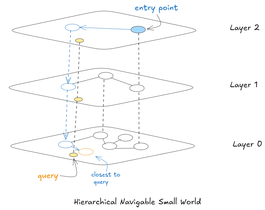
HNSW, proposed by Malkov and Yashunin in 2016, solves both NSW problems by borrowing the skip list’s idea of layers and applying it to the graph. Instead of one flat graph, you get multiple layers stacked on top of each other. Layer 0 at the bottom has every single vector, densely connected to nearby neighbors. Each layer above has fewer nodes with longer-range connections. The top layer might have only a handful of nodes spread across the entire vector space.

Think of it like Google Maps routing. Planning a cross-country drive street-by-street from the start would be insane. Maps zooms out first, picks highways to get you to the right state, then major roads to get you to the right city, then finally local streets for the last stretch. HNSW does the same thing. Upper layers are the highways, big jumps across vector space. Layer 0 is where you slow down and do the precise final search.

How Layers Are Assigned

Every time a new vector is inserted, it gets randomly assigned a maximum layer level using this formula from the paper:

level = floor(-ln(random()) * mL)

random() is a uniform random number between 0 and 1. mL is 1 / ln(M) where M is the max neighbors per node. The floor just rounds down to a whole number.

The reason this specific formula was chosen is that it produces the same kind of layered distribution as a skip list. The -ln(random()) part follows an exponential distribution, which means small values (layer 0, 1) come up very often and large values come up very rarely. Multiplying by mL scales that to match how many layers make sense for a given M.

Concretely, with M = 16, the probability of a node reaching layer l is exactly (1/16)^l:

• Layer 0: every node lives here
• Layer 1: 1/16 of nodes reach here (~62 out of 1000)
• Layer 2: 1/256 of nodes reach here (~4 out of 1000)
• Layer 3: 1/4096 of nodes reach here (essentially zero)

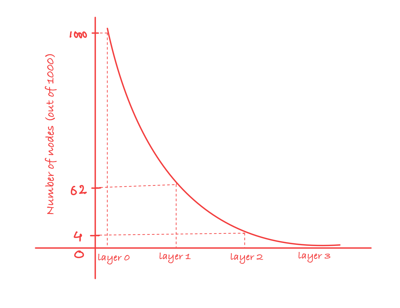
Each layer has roughly 16x fewer nodes than the one below it. This is what keeps upper layers sparse enough to be useful as fast navigation lanes, and it’s also what fixes the hub problem from NSW. Since layer assignment is random and happens at insert time, nodes inserted early have no special advantage. A node that was the very first insertion is just as likely to sit only at layer 0 as one inserted last.

This is what actually fixes the hub problem from NSW. Since layer assignment is random, a node inserted first has no special advantage over one inserted a million insertions later. The graph stays balanced on its own.

In our Rust implementation this looks like:

pub struct LevelGenerator {
    pub level_scale: f64,
}

impl LevelGenerator {
    pub fn from_m(m: usize) -> Self {
        // mL = 1 / ln(M), the scaling factor
        let level_scale = 1.0 / (m as f64).ln();
        Self { level_scale }
    }

    pub fn sample_level(&self, rng: &mut impl Rng, max_layer: usize) -> u8 {
        let u: f64 = rng.random().clamp(f64::EPSILON, 1.0 - f64::EPSILON);

        let l = ((-u.ln()) * self.level_scale).floor() as usize;

        // saturating_sub(1) just means "subtract 1 but don't go below 0"
        l.min(max_layer.saturating_sub(1)) as u8
    }
}

Three small things worth noting here. level_scale is computed once when the index is created, not on every insertion which saves a ln() call on every write, which adds up. The clamp on u is a safety guard, since ln(0) would give -inf and crash. And the level cap keeps the graph from growing extra empty layers that waste memory without helping search.

Usage looks like:

// at index init
let level_generator = LevelGenerator::from_m(max_connections);

// at each insertion
let l = index.level_generator.sample_level(&mut rng, index.max_layer);

The M Parameter

M controls how many neighbors each node connects to at each layer. Higher M → denser graph → better recall, more memory, slower inserts. Lower M → sparser graph → faster to build, lower recall. Typical production values:

• M = 8 — memory-constrained environments
• M = 16 — general purpose default
• M = 32–64 — high-recall requirements where memory isn’t a concern

There’s also M0, the connection count specifically at layer 0. The paper defaults this to 2 * M because layer 0 is where precision search actually happens, so you want it denser than the upper layers.

In Part 2 we get into the actual algorithms: how INSERT navigates layers to find the right neighbors, how SEARCH uses ef to trade speed for recall, soft delete, rebuild, and how we implemented all of this in Rust for VortexDB.