Implementing HNSW index (Part 2)
Part 1 covered the mental model behind HNSW: the layered graph structure, random level assignment, and why it works. This post walks through the actual implementation: insert, search, soft delete, and rebuild in VortexDB, a vector database in Rust we are building at SDSLabs.
Defining the index structure
Before writing any algorithm, you need to decide what the index actually holds in memory.
The Node
Each vector in the index is represented as a Node. A node stores:
- its own ID
- the highest layer it lives on
- a neighbor list per layer
- a deleted flag for soft deletes
struct Node {
    id: PointId,
    level: u8,
    neighbors: Vec<Vec<PointId>>,  // neighbors[layer] = list of neighbor ids
    deleted: bool,
}
The graph store
The graph itself is held in a PointIndexation struct:
struct PointIndexation {
    max_connections: usize,      // M
    max_connections_0: usize,    // M0, typically 2 * M
    max_layer: usize,
    points_by_layer: Vec<Vec<PointId>>,  // which nodes exist at each layer
    nodes: HashMap<PointId, Node>,
    entry_point: Option<PointId>,
    level_generator: LevelGenerator,
}
points_by_layer[l] holds the IDs of every node that lives at layer l or above. It gets updated on every insert: when you insert a node with level l, you append its ID to points_by_layer[0] through points_by_layer[l]. This lets rebuild quickly collect all nodes at a given layer without scanning every node in the graph.
The index
The top-level HnswIndex wraps the graph store and adds:
ef_construction: beam width used during insertef: beam width used during searchcache: aHashMap<PointId, Vec<f32>>holding the actual vectors in memorysimilarity: the distance metric, fixed at creation time
struct HnswIndex {
    ef_construction: usize,
    ef: usize,
    index: PointIndexation,
    data_dimension: usize,
    cache: HashMap<PointId, Vec<f32>>,
    similarity: Similarity,
}
In VortexDB we default to M = 16, M0 = 32, ef_construction = 200, ef = 100, and a max of 16 layers. The cache is fully in-memory for now. If your dataset is larger than available RAM, the standard approach is to back the vector cache with persistent storage and fetch on cache miss.
INSERT
The HNSW paper (Malkov & Yashunin, 2018) describes insert in Algorithm 1. It has two clearly separated phases.
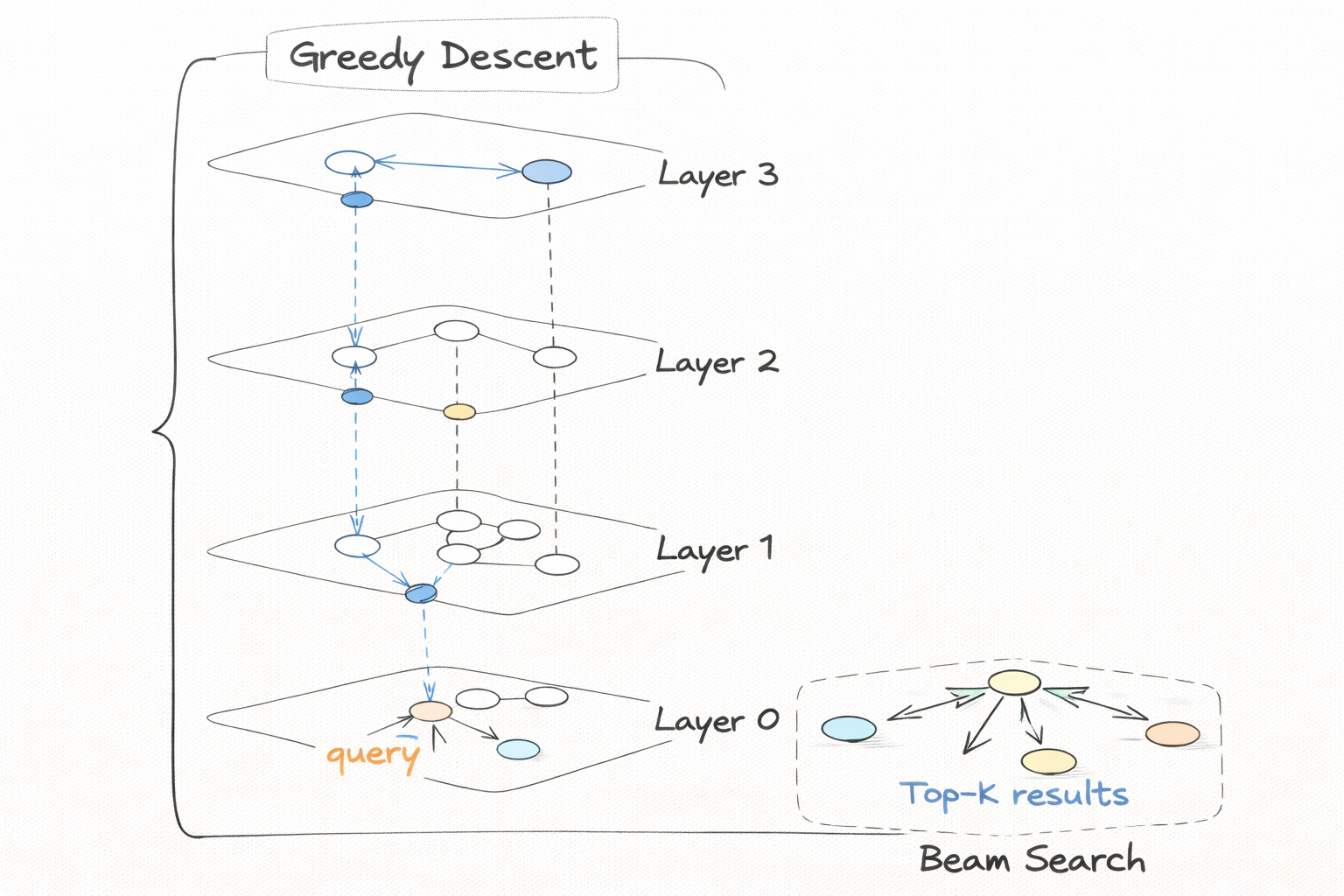
Phase 1: navigate to the right neighborhood.
The new node gets a sampled level l. Say the graph already has nodes up to layer 6 but the new node only reaches layer 2. Starting from the global entry point at the top of the graph, you descend one layer at a time from layer 6 down to layer 3 (l + 1), doing a greedy single-node walk at each layer. Greedy here means: look at your current node’s neighbors at this layer, move to whichever one is closer to your query, repeat until nothing improves, carry that node down to the next layer. One node is enough at this stage because you are only trying to get into the right region of the graph. Running a full beam search at every layer above l would be slow and unnecessary.
Phase 2: build connections.
Now you are at layer l. For each level from l down to 0:
- Run a beam search (width
ef_construction) to collect the best candidate neighbors - From those candidates, pick at most
Mneighbors using the diversity heuristic - Wire the new node to those neighbors bidirectionally
- Take the closest result as your entry point for the next level down
At layer 0 you use M0 connections instead of M because that is where the final precision search happens and you want it denser.
The main insert loop in pseudocode:
fn insert(new_id, query_vec) {
    let l = level_generator.sample_level();

    // first insert: just set it as entry and return
    if entry_point is None {
        entry_point = new_id;
        entry_point_level = l;
        return;
    }

    let mut ep = entry_point;

    // Phase 1: greedy descent for layers above l
    // current_max_level is the level of the current entry point node
    for level in (l+1 ..= current_max_level).descending() {
        ep = greedy_search_layer(ep, level, query_vec);
    }

    // Phase 2: beam search + connect at each level from l down to 0
    for level in (0 ..= l).descending() {
        let candidates = search_layer(ep, level, query_vec, ef_construction);
        let m = if level == 0 { M0 } else { M };
        let chosen = select_neighbors_heuristic(candidates, m);
        connect_bidirectional(new_id, chosen, level, m);
        ep = candidates[0]; // closest result seeds the next level
    }

    // update points_by_layer for the new node
    for layer in 0 ..= l {
        points_by_layer[layer].push(new_id);
    }

    // new node becomes entry point only if it reached a strictly higher layer
    if l > current_max_level {
        entry_point = new_id;
        current_max_level = l;
    }
}
current_max_level here is the level of the current entry point node, not a separate counter. When the new node’s level is strictly greater, it becomes the new entry point and current_max_level gets bumped. If l == current_max_level, both nodes live at the same top layer and the existing entry point stays.
Now let’s go through each of the four internal functions in the order you would implement them.
greedy_search_layer
This is the simplest of the four. Used in both insert phase 1 and the top layers of search.
What it does:
- Start at node
epat the given layer - Look at every neighbor of the current node at that layer
- If any neighbor is closer to the query, move there
- Repeat until no neighbor is an improvement
- Return the final node
greedy_search_layer -- click to see implementation
fn greedy_search_layer(ep, level, query) -> NodeId {
    let mut current = ep;
    loop {
        let mut best = current;
        for neighbor in current.neighbors[level] {
            if neighbor.deleted { continue; }
            if distance(neighbor, query) < distance(best, query) {
                best = neighbor;
            }
        }
        if best == current { break; } // no improvement, we are done
        current = best;
    }
    return current;
}
Skip deleted nodes during neighbor iteration. This is one place where soft deletes matter: a deleted node might still sit in a neighbor list (we never rewrite those), so you check the deleted flag before considering it.
This returns exactly one node, not a set. That is intentional for phase 1. The goal is to get to the right neighborhood fast, not to exhaustively explore the layer.
search_layer (beam search)
This is the core of phase 2, and we use this exact same routine during search as well.
What it does:
- Run a best-first beam search starting from
epat the given layer - Maintain two collections:
candidates: a min-heap (closest first), unbounded, tracks what to explore nextresults: a max-heap (farthest on top), bounded toef, tracks best found so far
- Expand the closest candidate, look at its neighbors, add unvisited ones to both heaps
- If
resultsis full, evict the farthest before inserting a better one - Stop early when the closest remaining candidate is farther than the worst result already in the set
search_layer -- click to see implementation
fn search_layer(ep, level, query, ef) -> Vec<(NodeId, f32)> {
    let visited = {ep};
    let candidates = min_heap with ep;  // sorted by distance, small = top
    let results = max_heap with ep;     // sorted by distance, large = top, capped at ef

    while candidates is not empty {
        let (best_dist, current) = candidates.pop_min();

        // early exit: nothing left to explore can improve results
        if results.len() >= ef && best_dist > results.peek_max() {
            break;
        }

        for neighbor in current.neighbors[level] {
            if neighbor in visited or neighbor.deleted { continue; }
            visited.insert(neighbor);

            let d = distance(neighbor, query);
            if results.len() < ef || d < results.peek_max() {
                candidates.push(neighbor, d);
                results.push_or_replace(neighbor, d);  // evict worst if full
            }
        }
    }

    return results sorted by ascending distance;
}
The early exit is the most important part. Without it, the beam search degrades to a full graph traversal on large layers. With it, you stop as soon as you can prove that no remaining candidate can improve your current result set.
ef_construction and ef are both passed into this same function. ef_construction is used during insert to build a well-connected graph. ef is used at query time and is your recall/speed knob: higher ef means better recall at the cost of slower queries.
select_neighbors_heuristic
Given the candidate set from the beam search, you need to pick at most M of them as actual neighbors for the new node.
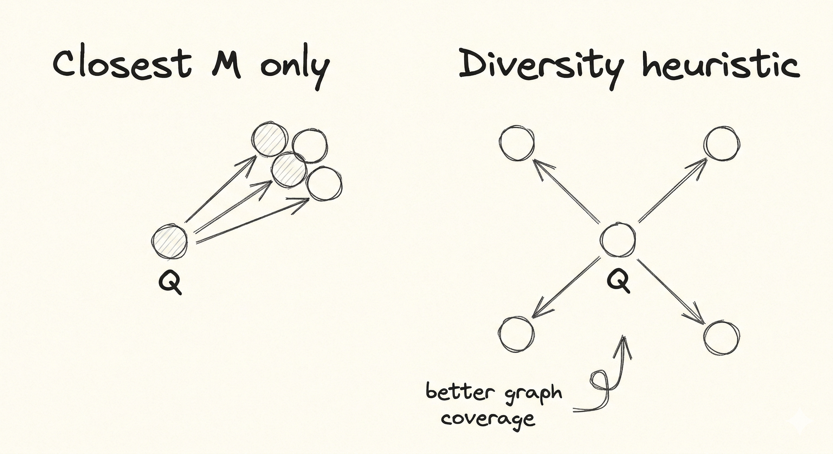
Why not just pick the closest M?
The problem is clustering. Suppose the beam search found 50 candidates and the 10 closest are all in the same dense region of vector space, very near each other and very near the new node. Connecting to all 10 wastes edges because all 10 point into roughly the same direction. You get better search coverage by spending some of those edges on nodes that point in different directions.
How the heuristic works:
Go through candidates in order of distance to the new node (closest first). For each candidate, check whether any already-accepted neighbor is closer to that candidate than the candidate is to the new node. If yes, the accepted neighbor already covers that direction, so this candidate is redundant and gets skipped.
Say the new node has these 4 candidates after beam search:
| Candidate | Distance to new node |
|---|---|
| A | 0.3 |
| B | 0.4 |
| C | 0.5 |
| D | 0.9 |
- A is accepted first, result is empty so nothing to compare against.
- B: distance to new node is 0.4, but distance from B to A is 0.1. Since 0.1 < 0.4, A already covers this direction. B is skipped.
- C: distance to new node is 0.5, distance from C to A is 0.6. Since 0.6 > 0.5, A does not cover C. C is accepted.
- D: same check passes. D is accepted.
Result is [A, C, D] instead of the naive [A, B, C], which fans out better across the vector space.
select_neighbors_heuristic -- click to see implementation
// candidates is a list of (NodeId, distance_to_new_node) pairs
fn select_neighbors_heuristic(candidates, m) -> Vec<NodeId> {
    let sorted = candidates sorted by distance ascending;
    let result = [];

    for (cand_id, cand_dist) in sorted {
        // cand_dist is the distance from cand_id to the new node being inserted
        let dominated = false;
        for accepted in result {
            // if an already-accepted neighbor is closer to this candidate
            // than the candidate is to the new node, skip this candidate
            if distance(cand_id, accepted) < cand_dist {
                dominated = true;
                break;
            }
        }
        if not dominated {
            result.push(cand_id);
        }
        if result.len() == m { break; }
    }

    return result;
}
The result is a set of neighbors that naturally fans out in different directions from the new node. This is a big reason HNSW gets high recall even with small M values.
connect_bidirectional
After selecting neighbors, you need to wire the new node to each of them in both directions.
What it does:
- Add the chosen neighbors to the new node’s neighbor list at this level
- For each chosen neighbor, add the new node to that neighbor’s list at this level
- If a neighbor’s list is now over its cap (
MorM0), prune it down
The pruning step for existing nodes uses simple distance-based truncation:
connect_bidirectional -- click to see implementation
fn connect_bidirectional(new_id, neighbors, level, m) {
    // connect new node to its neighbors
    new_id.neighbors[level] = neighbors;

    // connect each neighbor back to new_id
    for neighbor_id in neighbors {
        neighbor_id.neighbors[level].push(new_id);

        // if over cap, prune by distance from neighbor_id to each of its neighbors
        // (keep the closest m neighbors to neighbor_id, drop the rest)
        if neighbor_id.neighbors[level].len() > m {
            re-score each entry by distance(neighbor_id, entry);
            sort ascending;
            truncate to m;
        }
    }
}
The pruning uses distance from neighbor_id to each of its current neighbors, not distance to the query or to new_id. You are trimming neighbor_id’s own neighbor list, so what matters is which nodes are closest to neighbor_id itself.
We use simple truncation here instead of re-running the full diversity heuristic. The diversity heuristic was already applied when those neighbors were originally inserted, so the list was already reasonably spread out. Re-running it on every affected list on every insert would be expensive.
SEARCH
Search is simpler to implement than insert once you have the beam search working.
How it works
Search reuses two functions you already wrote: greedy_search_layer and search_layer. The structure mirrors insert exactly.
Phase 1: Greedy single-node descent from the global entry point at the top layer, down to layer 1. Same as insert phase 1, but descending all the way to layer 1 instead of stopping at l + 1.
Phase 2: One thorough beam search at layer 0 only, using max(ef, k) to ensure you always explore at least as many candidates as you are returning.
fn search(query, k) -> Vec<PointId> {
    let ep = entry_point;

    // Phase 1: greedy descent from top layer to layer 1
    for level in (1 ..= current_max_level).descending() {
        ep = greedy_search_layer(ep, level, query);
    }

    // Phase 2: beam search at layer 0
    let ef0 = max(ef, k);
    let candidates = search_layer(ep, 0, query, ef0);

    return candidates[..k]; // top-k by distance
}
Layer 0 gets the thorough search because it has every node in the graph and the densest connections. The upper layers are just navigation. All the precision comes from layer 0.
Tuning ef
The single knob that controls the recall/speed tradeoff at query time is ef. It is the beam width passed to search_layer at layer 0.
- Higher
ef: explores more candidates, higher chance of finding the true nearest neighbors, slower per query - Lower
ef: faster queries, lower recall
A useful way to think about it: ef is the minimum result set size you are willing to consider before stopping. The early-exit condition in the beam search means you might stop before visiting all ef nodes, but you will never return fewer than ef candidates (unless the graph itself has fewer nodes).
In practice, ef between 50 and 200 covers most use cases. Benchmark against your actual data and pick the point where recall@k stops improving.
Soft delete and rebuild
Why soft delete
Structurally removing a node from an HNSW graph is expensive. You would need to find all nodes that have it in their neighbor lists, remove it from those lists, and potentially re-run neighbor selection for each affected node to fill the gap. Across multiple layers, for a single deletion, this is a lot of work.
Instead, we mark the node as deleted and remove its vector from the cache. That is the entire delete operation. Every traversal already checks the deleted flag and skips those nodes.
fn delete(id) {
    node.deleted = true;
    cache.remove(id);

    // if this was the entry point, pick the next best
    if entry_point == id {
        entry_point = pick_highest_level_non_deleted_node();
    }
}
The deleted nodes stay in the graph structure. Their neighbor lists still exist. The edges that pointed to them are now dead ends that get skipped during traversal. From any caller’s perspective the node is gone.
Dead nodes accumulate in memory and create dead-end edges in the graph. As more nodes get deleted, search quality gradually drops because some paths through the graph now terminate early at deleted nodes rather than continuing to real candidates. This effect is mild for moderate delete rates (under ~20%) but becomes noticeable beyond that.
Tracking when to rebuild
VortexDB exposes a deleted_ratio() method:
fn deleted_ratio() -> f32 {
    deleted_count / total_count
}
The caller polls this and decides when the ratio is high enough to justify a rebuild. A reasonable threshold is 20-30%.
Rebuild
When the deleted ratio crosses the threshold, a full rebuild clears the graph and reinserts everything from scratch:
fn rebuild_full() {
    // collect all surviving vectors before wiping anything
    let survivors = all non-deleted (id, vector) pairs from cache;

    // wipe the graph entirely
    nodes.clear();
    points_by_layer.clear();
    entry_point = None;
    cache.clear();

    // reinsert from scratch
    for (id, vec) in survivors {
        insert(id, vec);
    }
}
Collect survivors before cache.clear(). If you clear first, you lose the vectors and have nothing to reinsert. Also keep an exclusive write lock for the whole rebuild, so readers never observe a partially rebuilt graph.
This re-runs a full insert for every surviving node, so you pay ef_construction beam searches per node across all their layers. For a large index this is expensive. But it fully restores graph quality because the new graph is built from scratch with no dead edges.
The full implementation with all the error handling, type wrappers, and distance metric plumbing is in VortexDB. The code is organized across types.rs (structs), index.rs (insert, delete, search, rebuild), and search.rs (all the layer traversal helpers).